Gradient Descent is an optimisation algorithm for finding the local minimum of a function. It searches for the combination of parameters that minimises the cost function. For the Gradient Descent to work, the cost function must be differentiable and convex.

Steps

1. A hypothesis function is defined and its weights or coefficients are initialised: small random values or zeroes are assigned to the weights or coefficients (θ₀, θ₁...). $$ h_\theta(x) = \theta_0 + \theta_1 x $$

   Example of hypothesis function

2. The dependent variable of the hypothesis function is calculated using those coefficients for each data input.

3. The cost function (sum of the squared residuals) is computed:

   $$ J = \frac{1}{2m} \sum_{i=1}^{m} (h(x^{(i)}) - y^{(i)})^2$$

   Cost function. Rigorous version here

4. Compute the gradients: partial derivatives of the cost are calculated to find the direction that minimises the cost function. $$\frac{\partial}{\partial \theta_j} J(\theta_0, \theta_1)$$

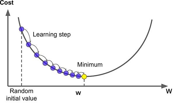
   Computation of gradients

5. Move in the direction opposite to the gradients: the learning rate parameter (α), which is a scale factor that controls how much the coefficients change from one iteration to another, is applied to the gradients and this is subtracted to the coefficients, which are then updated.

   $$ \theta_j := \theta_j - \alpha \frac{\partial}{\partial \theta_j} J(\theta_0, \theta_1)$$

   Update the coefficients

6. The process from the second step is repeated until the minimum error is achieved or no further improvement is possible.

Types of Gradient Descent

There are three different ways of computing the Gradient Descent:

Batch Gradient Descent

• It uses the whole training data to compute the gradients at every iteration and update the coefficients.
• The optimal solution is reached smoothly.
• This approach is very computationally expensive since the entire dataset needs to be loaded and all operations performed on that.

Stochastic Gradient Descent

• It selects a random instance in the training data at every iteration to compute the gradients on that single instance and update the coefficients.
• The optimal solution is reached after many iterations since the data used can be very different in each step.
• The computational cost is lower than the Batch Gradient Descent, as only one instance is computed at each iteration. However, many more iterations will be required.

Mini-batch Gradient Descent

• It is in the middle between the previous two ways, as it selects a small set of random instances at every iteration to compute the gradients and update the coefficients.
• The optimisation process is less noisy than in the stochastic Gradient Descent because we use more instances for updating the coefficients, but not as smooth as in the batch Gradient Descent.
• The computational cost is the lowest of all methods, since we are loading only a set of the data and a lower number of iterations are required.

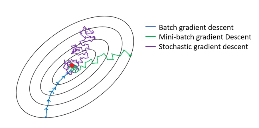
Batch Gradient Descent is the one that takes less time to find the solution, but it requires a lot of resources. Stochastic Gradient Descent is computationally light, but it requires many iterations to find the optimal solution. Mini-batch Gradient Descent lies in the middle.

If you liked this content don't forget to follow me here and on Twitter!