When working with time series data, it is important to assess the quality of a model in a way that accurately reflects real-world situations.

Generally, the simplified process of building a Machine Learning model is the following:

1. Process and clean your data

2. Train the model using your training set

3. Evaluate and assess its performance with the testing set

This is the way it is traditionally done in Data Science. However, when dealing with Time Series data, there is a better approach. This approach consists of repeating the last two steps to consider all available information at the time.

Using the traditional method of forecasting will miss important information already known. A better approach is to use a method called “Rolling window forecast”.

Rolling window forecast

This method involves gradually adding one value from the test set to the training set at a time, training a new model on the updated training set, and using the model to predict the next value in the test set. This process is repeated until the entire test set has been predicted.

For example, let’s say you are working with daily sales data and your training set ranges from 2015 to 2021, and a testing set covering the entire year of 2022. You would train your model (ARIMA model in this example) using the training set and then gradually add one value from the test set to the training set, train a new model on the updated training set, and use the model to predict the number of sales for the next day in 2022.

This method is considered to provide a more accurate evaluation of the model’s performance and allows you to see how the model would perform in real-world situations. Additionally, it helps in considering all available information to make predictions.

# Define model order and number of steps
order = (1,1,1)
steps = 10

# Initialize predictions array
predictions = []

# Loop through time periods
for step in range(steps): 

    # Add new prices to the previous ones
    prices_train_i = pd.concat((prices_train, prices_test[:step]), axis=0)

    # Train new model
    model_i = ARIMA(prices_train_i.values, order=order).fit()

    # Forecast next day price
    pred = model_i.forecast(steps=1)

    # Add to predictions array
    predictions.append(pred)

# Create dataframe
df_rolling = pd.DataFrame(predictions, index=prices_test[:steps].index)

It is important to note that there are two different ways of using the rolling window forecast:

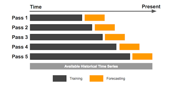
• Fixed or sliding rolling window: the same size of window is used throughout the forecast process. For example, if a fixed window of size 12 is used, the model will be trained on the first 12 data points, then the next 12 data points, and so on. The model is retrained with new data every time the window slides. This method is useful when the data is relatively stable and the patterns in the data do not change significantly over time.

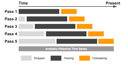
• Expanding rolling window: the window size increases as the forecast process progresses. For example, the model may be trained on the first 12 data points, then the first 24 data points, then the first 36 data points, and so on. The model is retrained with new data every time the window expands. This method is useful when the data is evolving over time and the patterns in the data are changing.

Traditional or Multi-step forecast

In contrast, the traditional way of forecasting in Time Series, also known as multi-step forecast, consists of training the model once, with all available data until that moment, and then forecasting for several days in the future. However, this method may not take into account important data such as the evolution of the price from the training day until the present day.

# Define model order and number of steps
order = (1,1,1)
steps = 10

# Train ARIMA model
model = ARIMA(prices_train.values,
    order=order).fit()

# Forecast the future price values
df_traditional = pd.DataFrame(
    model.forecast(steps=steps),
    index=prices_test[:steps].index
)

Forecast comparison

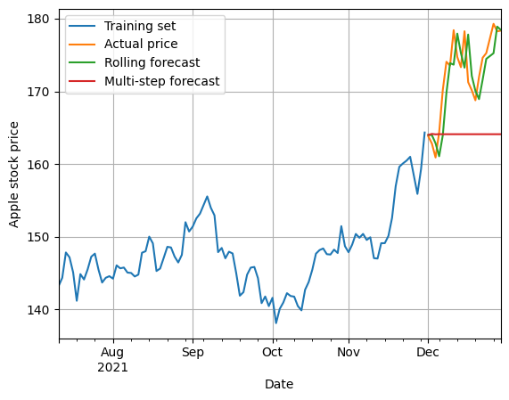
We will consider the previous example, in which we were trying to forecast the price of Apple stock.

We can see that the prediction made by the rolling (expanding window) forecast method is much closer to the actual price than the traditional forecast method. The traditional or multi-step one manages to predict only the first period or if the price does not change much, also the second period.

In conclusion, it is important to be aware of the different ways of forecasting future values in Time Series and to choose the method that best suits the problem at hand. The Rolling window forecast method is a better alternative to the traditional method as it provides a more accurate evaluation of the model’s performance and takes into account all available information. However, it requires the model to be retrained constantly, and this may not be ideal for your particular application.

Time Series articles

1. Introduction to ARIMA models

2. Parameters selection in ARIMA models

3. Seasonal ARIMA

4. ARCH / GARCH models for Time Series

5. ARIMA-GARCH models

6. Forecasting in Time Series