Parameters selection in ARIMA models
Time Series Forecasting - Part II

I am a Data Scientist. I write about Machine Learning, Data Science and Python.
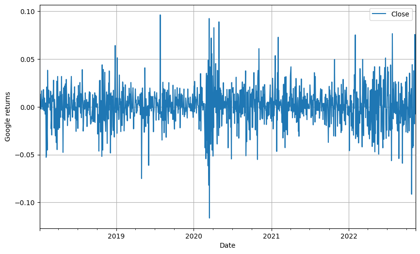
ARIMA models are a simple but powerful way of modelling time series. We saw that in the previous part.
An ARIMA(p,d,q) model is defined by three parameters:
p : autoregressive order
d : difference order
q : moving average order
What p, q and d parameters should we use?
How can we estimate d?
As seen in the previous article, we need a stationary model.
The statistical test employed to verify the stationarity of time series data is the Augmented Dickey-Fuller Test.
The hypotheses for this test are
H₀ (Null hypothesis) = Time series non-stationary
H₁ (Alternative hypothesis) = Time series is stationary
We need to define a significance level α, which is generally set to 0.05. This is used to compare it with the p-value from the test. On the one hand, if the p-value of the test is larger than the significance level, we fail to reject the null hypothesis, which means that our time series is non-stationary. On the other hand, if the p-value is lower than the significance level, we reject the null hypothesis, which for us means that our time series can be considered stationary.
To select d we will perform the test on the time series data. If we can conclude that it is stationary, then d is equal to 0. If it is not, we will need to apply a differencing transformation and check again. If after one differencing we achieve stationarity, then d would be equal to 1. This process should be repeated until defining d.
How can we estimate p and q?
We need to check how correlated the time series are with lagged versions of itself.
The original time series will be denoted as 0. A 1-timestep lagged version will be referred to as 1. And so on... The correlation of the original time series with the lag 0 (no lagged), will always be equal to 1 since they are the same time series.
We need to differentiate two correlations:
The indirect correlation that the timestep t-1, t-2, t-3… have over timestep t, just by being adjacent to one another. For example, with stock prices, the price today will be influenced by the price it had yesterday. Also, the price yesterday will be affected by the price the day before.
The direct correlation that each of the previous timesteps has over timestep t. Following this example, imagine that every three days there is a special event, it is expected that we will see a direct correlation of the time series with a lag 3 series.
To measure these two effects we can use the ACF and PACF graphs:
**ACF **(AutoCorrelation Function) shows the correlation between timesteps. It includes both direct and indirect effects.
**PACF **(Partial AutoCorrelation Function) shows only the direct correlation.
We use the so-called "lollipop" graphs to visualise it.
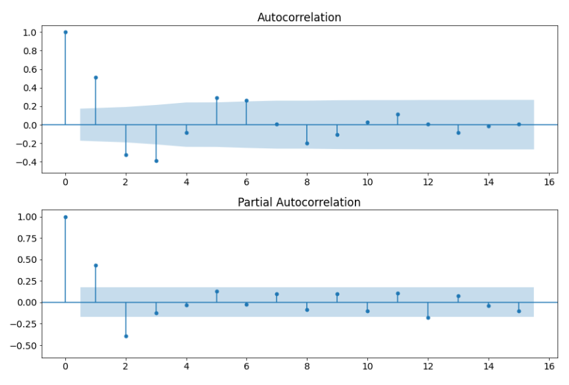
There are several spikes or "lollipops" on it. They indicate the correlation of each lag (on the x-axis) with the original non-lagged time series. We will pay attention to the largest spikes closer to lag 0 that are outside the blue-shaded area. If a spike lies in this area, it would mean that its correlation is not significantly different from 0 and therefore not relevant.
For the p parameter, which determines how many previous values we need to consider for the Auto-Regressive part of ARIMA, we need to check the PACF graph as we are interested in the direct correlation.
For the q parameter, which determines how many previous residuals we need to consider for the Moving Average part, we need to check the ACF graph as we want the direct correlation.
Build your own model
If you want to know how to build your own model, you can follow the step-by-step guide I shared on Twitter:
If you liked this content don't forget to follow me here and on Twitter!