ARIMA-GARCH models

ARCH/GARCH models can assist or improve the forecast of ARIMA models.

Firstly, time series data must be stationary for these models to be applicable. If not, we should apply some transformations such as differencing. Since these models are mainly used in finance we will refer to the price returns from now on, which are the result of applying differencing to the share prices.

Returns (rₜ) can be modelled as:

$$r_t=\mu_t + \varepsilon_t$$

It can be decomposed into two components:

• Mean (μₜ): this can be represented by an ARIMA model.

• Error term (εₜ): this refers to the residuals after fitting a mean model such as ARIMA. For certain applications like finance, the variance may change consistently over time, with periods of high or low volatility, also called volatility clustering. ARIMA models are not capable of capturing these variance or volatility changes over time, which we call heteroskedasticity. This can have a big impact on certain applications, for example in assessing the risk of investments. If this change in variance is autocorrelated over time, ARCH/GARCH models can be used to capture it.

ARCH/GARCH models

ARCH/GARCH models expect the series to be stationary and with no other components such as trend or seasonality, only change in variance. Let's remind the differences between them:

• ARCH models the change in variance over time as a function of the residual errors from a mean process.

• GARCH models are an extension of the ARCH models that incorporate a moving average component together with the autoregressive component. In addition to the lag residual errors, it also includes the lag variance terms from a mean process.

These models have two main applications:

1. Forecast volatility

2. Consider the variance of the ARIMA residuals to improve the forecast

Volatility forecast

We can assume a constant or zero mean for the returns and fit directly an ARCH/GARCH model.

These are the steps to follow:

1. Get the returns (percentual change) from the data

2. Estimate the parameters "q" for ARCH models or "q" and "p" for GARCH models by plotting the PACF of the squared returns

3. Test higher-order models to find the one that minimises the AIC

4. Forecast volatility!

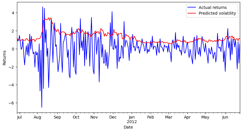
Below you can see the volatility forecasts after fitting an ARCH(11) model on the S&P500 price returns.

ARIMA-GARCH model

An ARIMA-GARCH model will take into consideration the change in variance to improve the prices or returns forecast.

The steps to follow are:

1. Get the returns (percentual change) from the data

2. Fit an ARIMA model:

   1. Find optimal "p" and "q" parameters

   2. Fit model on training data

   3. Compare with actual returns to get residuals

3. Check for heteroskedasticity in the residuals. For example, checking the PACF of the squared residuals. Also, we could use Ljung–Box test or the Lagrange Multiplier test.

4. Fit an ARIMA-GARCH model. We have two options here:

   1. Fit a GARCH model on the residuals of the ARIMA model and add both contributions.

   2. Fit both models simultaneously. This is the preferred way as otherwise, ARIMA estimates may be inconsistent.

5. Forecast the returns! You could also add accurate confidence intervals thanks to the variance modelling.

Build your own ARIMA-GARCH

In the following articles and on Twitter I will show how you can do this in Python.

So if you liked this content, don’t forget to follow me here and on Twitter not to miss out!